Fiber Detector
The fiber detector calculates the coupling efficiency of an incident field into a single-mode optical fiber. The coupling efficiency is defined as the “fraction of the power of the incident optical field mode that is coupled into the propagating mode of an optical system” [1]. Optiscan calculates the coupling efficiency using the overlap integral described in the important equations section. It should be noted that the coupling efficiency is always a number between 0 and 1, because it is the fraction of the incident power that is accepted by the fiber.
Getting Started:
Select Build -> Detectors -> Fiber in the main model panel.
Click on Arrange Object and drag the fiber detector ![]() to the desired position.
to the desired position.
Editing the Fiber Detector:
On opening the fiber detector icon for editing, the propagating mode patterns for X, Y, and Z polarizations are displayed. The default fiber detector in Optiscan is square-shaped with dimensions of (10 microns x 10 microns) and a sampled array size of (200×200). The default X and Y polarization mode patterns are single-mode Gaussians [2] with 1/e2 radii of 1.944 microns at a wavelength of 1550 nm, corresponding to a fiber core diameter of 5 microns. The indices of refraction for the core and cladding used in calculating the 1/e2 radius are nco = 1.5 and ncl = 1.4. The default mode pattern for the Z-polarization direction is zero, because the optical fields are presumed to be completely transverse to the axis of the fiber.
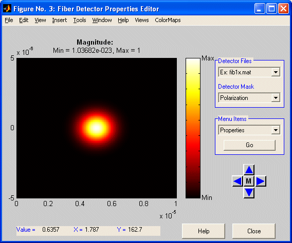
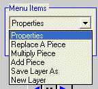
The size and sampling of the fiber detector can be reconfigured by the user by selecting the PROPERTIES menu item and clicking on GO. This opens the DETECTOR DIMENSIONS window. This window functions exactly like the DIMENSIONS windows for the SOURCE object, SIMPLE RESPONSIVITY DETECTOR, and the many TARGET objects. The size, offset and sampling rates can be easily reconfigured by the user. However, always remember to check your sample size so that the total array size of the detector is reasonable. For example, be careful not to have a detector whose size is 1cm x 1cm and whose sampling is 1e-7 x 1e-7, because this would result in an array size of 100000×100000, which is far too large for the computer. A good rule of thumb is to set the sampling such that the array size of the detector is between 100 x 100 and 1000 x 1000.
The propagating mode patterns of the FIBER DETECTOR may be reconfigured. The procedure for editing a propagating mode pattern is identical to editing the shapes of the SOURCE or TARGET objects. The user selects one of the editing options (replace a piece, multiply a piece, or add a piece) in the menu selection, and follows the instructions to build the desired propagating mode pattern. The user should note that the propagating mode pattern of the fiber is equal to
![]() (see Important Equations).
(see Important Equations).
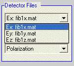
Unlike the SIMPLE RESPONSIVITY DETECTOR, the user may independently alter the mode patterns of the FIBER DETECTOR in the X,Y, and Z polarization directions.
The output data file for the detector can be changed by selecting the PROPERTIES menu item, and clicking on GO. When the new window appears, click on the RESULTS FILE tab in the upper section of the window.
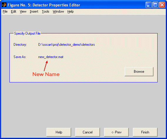
Note: if more than one fiber detector is used in a project, each output file must be named differently. This is done in the last step of editing the fiber detector propagating mode pattern. The user must uniquely specify the filename that the propagating mode pattern is saved under.
Using the Fiber Detector:
Once the desired detector pattern is generated, the user links the detector into the project workspace.
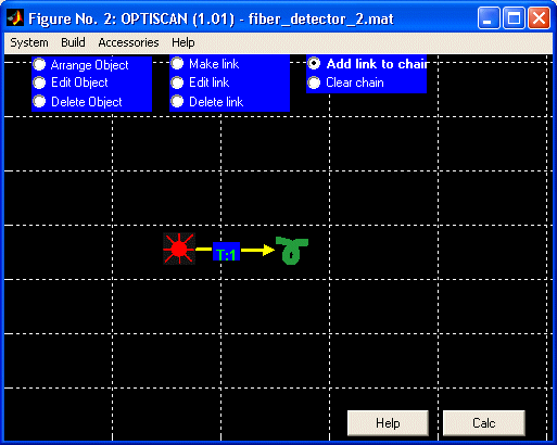
Running a simulation determines the amount of power transferred from the optical system to the fiber (i.e. the coupling efficiency). The format of the data file is a simple ASCII text file that is tab delimited. The following is a sample of how the data looks when imported into a spreadsheet:
| 3.52113298e-001 | 3.87943171e-001 | 3.95755503e-001 | 3.84127019e-001 | 15:32:43 |
| 3.52113298e-001 | 3.87943171e-001 | 3.95755503e-001 | 3.84127019e-001 | 15:32:47 |
| 3.52113298e-001 | 3.87943171e-001 | 3.95755503e-001 | 3.84127019e-001 | 15:32:50 |
| 3.52113298e-001 | 3.87943171e-001 | 3.95755503e-001 | 3.84127019e-001 | 15:32:53 |
The first three columns represent the coupling efficiencies resulting from the X,Y, and Z polarizations of the electric field incident upon the end of the fiber. The fourth column is the total coupling efficiency for all three polarizations together. The last column is a timestamp, which lets the user know at what time the data were taken.
Note that Optiscan will ONLY APPEND the detector data file, it will never overwrite it. This means that if the user wishes to perform a fresh simulation with no initial data in the output file, either the filename of the previous simulation needs to be changed, or the detector output filename must be changed or deleted.
Important Equations:
Coupling Efficiency

![]() represent the optical fields incident upon the fiber.
represent the optical fields incident upon the fiber.
![]() represent the complex conjugates of the propagating optical field modes inside the fiber.
represent the complex conjugates of the propagating optical field modes inside the fiber.
Gaussian Beamwidth of a Single-Mode Fiber (from Reference [2])
![]()
ω represents the 1/e2 radius of the propagating Gaussian fiber mode.
![]() where “a” is the radius of the fiber core, and “k” is the wave-number.
where “a” is the radius of the fiber core, and “k” is the wave-number.
 where
where ![]() is the propagating wavelength in air.
is the propagating wavelength in air.
Notes:
There is a slight bug that occurs when changing the mode pattern of the detector. The Y axis is reversed in the viewer that is used to select the window size and position for the new pattern element. This will cause an element positioned in the upper half of the screen in the edit window to actually appear in the lower half of the screen when the mode pattern is actually updated.
References
[1] K. Garcia, Calculating Component Coupling Coefficients. Laser Focus World. August 2000. Retrieved June 10, 2003.
<http://www.breault.com/ftp/docs/coupling.pdf>
A copy of this article is also available here.
[2] D. Marcuse, Loss Analysis of Single-Mode Fiber Splices, The Bell System Technical Journal, Vol. 56, No. 5, May-June 1977.
A copy of this article is also available here.

