

Quantum Control Lab
In the Quantum Control lab we are pursuing the general goals of quantum state preparation and quantum measurement of the internal states of Cesium atoms. We would like to build a set of experimental tools that allow us to create arbitrary quantum states within the ground state of Cesium and measure said states with high accuracy. Although specific goals in this lab may change over the years, a consistent recipe for every run of the experiment goes as follows:
- Create a cold, trapped gas of approximately one million Cesium atoms at 2 μK.
- Turn off all cooling and trapping fields.
- Atoms begin to free-fall due to gravity.
- Optically pump atoms to a known initial state.
- Drive quantum dynamics by applying laser and magnetic fields to evolve the initial state along a known trajectory.
- Make quantum state measurements using a projective measurement (Stern-Gerlach) or a continuous weak measurement (Faraday spectroscopy).
The bulk of our research goes into the specifics of steps 5 and 6. Currently our goals for these two steps are quantum control and quantum state tomography of the Cesium hyperfine ground manifold.
Quantum Control
Quantum control is jargon for the ability to prepare arbitrary quantum states within a defined state space. The state space we work in is the Cesium hyperfine ground manifold.
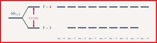 Fig. 1. Hyperfine structure of the Cesium ground state
The ground manifold consists of two hyperfine levels within 6S1/2 as shown above. This gives us a 16 dimensional state space to explore. Merkel et al [1] showed that a combination of static, radio frequency and microwave frequency magnetic fields allows for quantum control of the state space.
 Fig. 2. Control fields
Above is a cartoon of the applied fields in our experiment. A 1 MHz static field in the quantization direction, Z, Zeeman splits the magnetic sublevels. Radio frequency fields in X and Y with independent phase control allow for independent geometric rotations of the two hyperfine manifolds. A microwave field with phase control couples states |F=4, mF=4〉 and |F=3, mF=3〉. Given that all the fields have a fixed power, we can search numerically on a computer for the correct phases as a function of time to bring our initial state to a desired final state of our choice. We can show the results of these preparations with Stern Gerlach measurements.
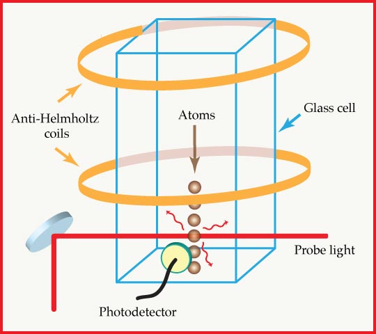 Fig. 3. Stern Gerlach measurement
Above is a cartoon of the Stern Gerlach device. The atom cloud starts as a cold gas in the center of the glass vacuum chamber. At the end of state preparation, the cloud falls through the gradient magnetic field created by a set of anti-helmholtz coils. The atoms split spatially based on their magnetic sublevel and fall though probes resonant with each hyperfine level. Atom fluorescence is detected by a photodiode and the populations in each sublevel can be determined.
Above left shows two Stern Gerlach measurments superimposed. In the background is atoms without any state preparation to show the 9 possible sublevels atoms can be in and the foreground shows atoms optically pumped to the state |F=4, mF=4〉. Above right shows the result of a state preparation of |F=4, mF=2〉.
Quantum State Tomography
Quantum state tomography is a process of determining the quantum state of a system. In our case, we have a large ensemble of non-interacting atoms. Although we would like the dynamics of each atom to be identical, in practice this is not possible due to spatial inhomogeneities in applied fields. In this case, we would like to know the density matrix for our ensemble. The experimental tool that allows us to gain information about the system is Faraday spectroscopy.
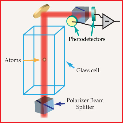 Fig. 4. Faraday spectroscopy setup
Above is a schematic of the Faraday spectroscopy setup. A linearly polarized probe beam is passed through the cold sample of atoms as the atoms are evolving. Depending on the state of the atoms and details of the probe intensity and frequency, the probe polarization will change. The probe is split by a polarizing beam splitting cube and sent to two ports of a differential detector. From these polarization changes, information about the quantum state can be inferred.
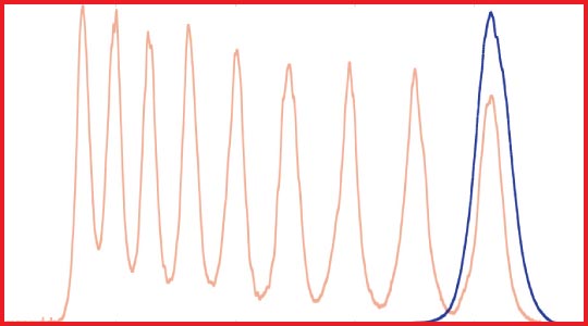
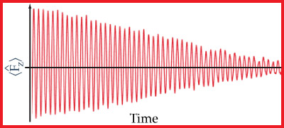 Fig. 5. Faraday spectroscopy signal
Above is a faraday spectroscopy signal. In this case, the atomic sample was spin polarized in a particular direction (Z) and an orthogonal constant magnetic field was applied. The spin larmor precesses and we can detect this precession by measuring the the amount the input linear polarization rotates due to the Faraday effect [2]. Thererfore, we can effectively measure a component of the spin operator, F, as a function of time. To perform quantum state tomography, consider reconstructing a state preparation. We apply a set of known control fields to this prepared state and constantly measure an expectation value of a component of the spin as the atomic ensemble evolves. Given this measurement record as a function of time, the known applied fields and an accurate Hamiltonian, this knowledge can be used to determine the initial prepared state.
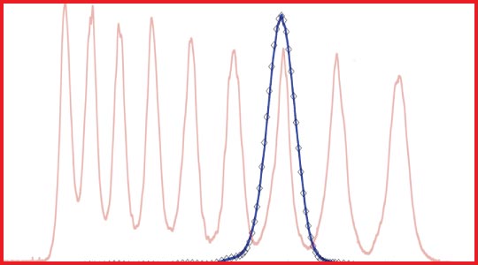
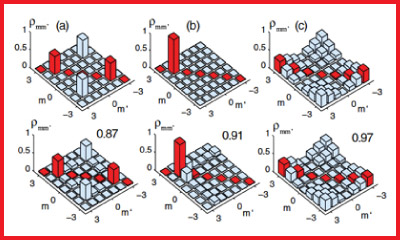 Fig. 6. Reconstructed density matrices
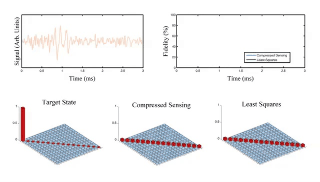
Above is a movie that illustrates the reconstruction procedure of a random pure state (expressed in a diagonal basis) utilizing two reconstruction computer algorithms. The figure on the top left shows the predicted signal using our model of the system and the blue line is the observed signal measured by the polarimeter in the experiment. The figure on the top right shows the fidelity of the reconstruction procedure as a function of time. In the bottom row we have the expected form for our reconstructed state (left) and the evolution of the density matrix as the information is obtained over the duration of the experiment for two distinct reconstruction algorithms (center and right).
[1] Merkel et al, Phys. Rev. A. 78, 023404 (2008).
[2] Smith et al., J. Opt. B: Quantum Semiclass. Opt. 5, 323-329 (2003).